📊 Understanding Matrix Multiplication
Matrix multiplication is one of the most computationally intensive operations performed in computers with vector processors. The multiplication of two n × n matrices consists of n² inner products or n³ multiply-add operations.
3 × 3 Matrix Example
Example Calculation: The element c₁₁ is calculated as:
This requires 3 multiplications and 3 additions (after initializing c₁₁ to 0)
⚡ Computational Complexity
For n × n matrices: The product of two n × n matrices requires n³ multiply-add operations. The computational complexity grows cubically with matrix size!
General formula: C = A₁B₁ + A₂B₂ + A₃B₃ + A₄B₄ + ⋯ + AₖBₖ
In typical applications, k may be equal to 100 or even 1000, making vector processing essential for performance.
🔄 Pipeline Vector Processing
The inner product calculation on a pipeline vector processor leverages parallel processing to dramatically improve performance.
Pipeline Architecture
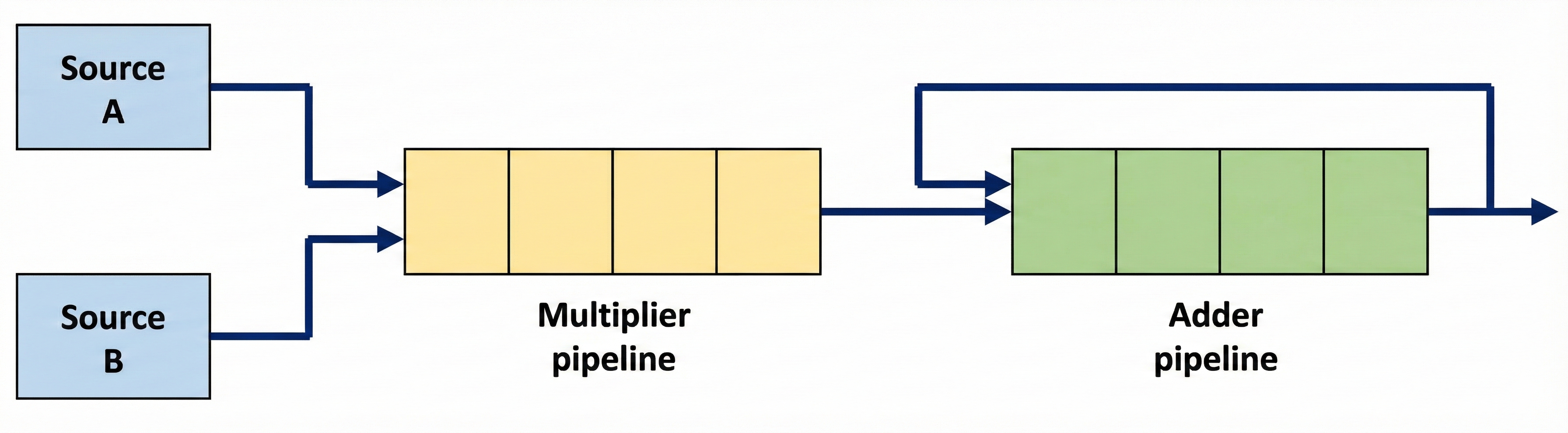
Pipeline Operation Stages:
+ A₅B₅ + A₆B₆ + A₇B₇ + A₄₄B₄₄ + ⋯
+ A₉B₉ + A₁₀B₁₀ + A₁₁B₁₁ + A₁₀B₁₀ + ⋯
+ A₄B₄ + A₈B₈ + A₁₂B₁₂ + A₁₆B₁₆ + ⋯
The summation breaks down into four parallel sections, each processing simultaneously through different segments of the adder pipeline.
🎯 Completion Phase
When there are no more product terms to be added, the system inserts four zeros into the multiplier pipeline.
The adder pipeline will then have one partial product in each of its four segments, corresponding to the four rows in the equation above.
The four partial sums are then added to form the final result.